
by Eric Brown –
In my last blog post, I reported my observations of a Health Care hackathon that was hosted by RCG, Pitney-Bowes, and the Technology Association of Georgia. That hackathon was so successful, that the same group held another hackathon—this time, focused on Financial Technology (FinTech.)
One of the areas that the contestants were allowed to choose from was how to repurpose ATM machines, given the fact that we are trending toward a cashless society, mostly mediated by credit and debit cards. Credit cards are so convenient, being nearly universally accepted, especially along the paths that business travelers frequently travel. In fact, I seldom carry cash, and so I seldom visit ATM machines.
Anyone who travels has likely experienced a certain anxiousness at a situation where they would hop off the plane in a place far from home, absolutely starving, but their credit card would not work. Would it be due to an overly aggressive fraud prevention algorithm with a rule that detects whether an account is accessed from two impossibly far locations? Should I call my spouse and ask her not to use the card until I’ve gotten my essentials squared away? In fact, rather than cash, I carry two credit cards, in case something goes wrong with my primary card. Suddenly, credit cards don’t seem so convenient. (And let me tell you how embarrassing it is on the rare occasions when my credit card has been declined.)
In spite of any inconvenience to a customer, businesses must be vigilant against fraud. How might we develop a methodology that effectively screens transactions and improves the bottom line of the business, while simultaneously keeping customers happy?
The Cost of (Mis)Classification
Consider a machine learning model that is trained to detect credit card fraud. In ML parlance, the situation that I just described (a false trigger) is called a False Positive (FP). There are three other situations: True Negative (TN, bona fide, normal transactions), True Positive (TP, cases of fraud detected), and False Negative (FN, cases of fraud escaping detection). When a large number of transactions are scored and classified by an machine learning model, it is common to summarize the performance of a model by a table that is called a Confusion Matrix:
| TN | FP |
| FN | TP |
where each element corresponds to the count of the number of successful classifications as predicted by the model, compared to what was actually observed, e.g. upon human verification.
A good model maximizes the number of TN and TP cases and minimizes the FN and FP cases (misclassification errors). Related to Specificity and Sensitivity, the most common metric reported is the Area Under the Curve (AUC) value, where values near ½ are as good as randomly guessing whether it is a fraud case, and values close to 1 are suggestive of highly-performant models.
In an overwhelming number of circumstances, both in textbooks and in practice, the performance of a model is evaluated where the cost of TN, FP, FN, and TP are taken to be equal. But in the case of credit card fraud, nothing could be farther from the truth! There are drastically different costs and benefits from each classification. In an approximate way, we can write the cost (positive number) and benefit (negative number) as:
| TN (Normal Transaction): | CTP = -1 x Transaction Amount x Merchant Fee |
| FP (Falsely Flagged Fraud): | CFP = Intervention Cost – Transaction Amount x Merchant Fee+ Customer Frustration |
| FN (Undetected Fraud): | CFN = Transaction Amount |
| TP (Detected Fraud): | CTP = Intervention Cost |
where it assumed that a Credit Fraud specialist would intervene if an machine learning model predicted a case of fraud, and it is further assumed that the credit card company would have to incur the full cost of any fraudulent transaction that was not caught. Substituting reasonable values into the above formulas reveals drastically different costs/benefits for each scenario, e.g. an average transaction amount of $100, and intervention cost of $5, a merchant fee of 1.5%, and an unspecified (though positive) cost of customer frustration, potentially leading to loss of all future revenue for that customer—a calamity, indeed—and not a remote probability if an honest customer’s transactions keep getting flagged a fraudulent!
Economists know this approach well: It is the optimization of cost-benefit (CB). In the next section, we will walk through an example of optimizing without consideration of CB, and gradually improve the decision-making model by including it.
A Practical Example – The Kaggle Credit Card Dataset
Financial Transactions contain highly personal information. However, they are among the most important data sets that data scientists consider. In order to provide insight into the performance of various models in light of the above costs, I have selected Kaggle’s famous “creditcard.csv” data set1 as a representative stream of transactions which may contain fraudulent usage. This dataset contains over a quarter million transactions, including a large number of possibly predictive variables, the amount of each transaction, and whether that case was indeed a fraud case. The average transaction value is around $90.
Strategy 1: Do Nothing
One thing to note about this data set is that the incidence of fraud is actually quite small, with a prevalence of only 0.1%. Before engaging in any sophisticated analysis, it is informative to summarize the amounts associated with normal and fraud cases:
| Case (N=Approx. Count) | Total Transaction Amount (Approx.) |
| Normal (N=280,000) | $25,000,000 |
| Fraud (N= 500) | $ 60,000 |
Could stop this exercise right now, and simply accept the loss? But in the above table, we have neglected to consider that the credit card transactor only receives a small portion of the transaction amount! Assuming the merchant fee is 1.5%, the normal transactions would net only $375,000, and suddenly the loss due to fraud ($60,000) is significant! Furthermore, it is human nature that, without a deterrent, crime would only increase. We’ve got to do something about it! Would statistical analysis be of help in figuring out which transactions are likely fraudulent?
Before doing so, let’s take a moment to write the costs of the “do nothing” strategy into a table which has the same form as the Confusion Matrix presented in the introduction:
| TN: -$375,000 (Normal Transactions) | FP: $0 |
| FN: $60,000 (Fraudulent Transactions Not Caught) | TP: $0 |
Summing the values of the table leaves us with a benefit of $315,000, making no effort in trying to correctly identify cases of fraud, and simply absorbing all the cost of fraudulent transactions.
Strategy 2: Logistic Regression
Perhaps the simplest model that we could construct for this problem is likely a logistic regression model. Logistic regression is virtually bullet-proof in execution, and the results that it obtains are often pretty good, provided that the relationship of the predictor variables and the outcome of interest is straightforward.
Once solved, Logistic Regression models afford a prediction of the probability that a particular transaction is fraudulent. The figure below shows the distribution of predictions of all the transactions:
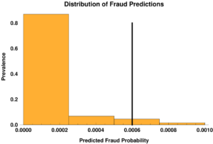
The plot also shows the optimal threshold (0.0006) for classifying a particular transaction as fraudulent, assuming that the costs of misclassification are the same for each TN, FP, FN, and TP. Cranking through the data set again, and accumulating the costs and benefits for each case, we determine that our bottom line is $285,000 – in fact, we lost money (compared to $315,000)!
In the next strategy, we would like to see if the problem is because the statistical method that we chose is simply a poor performer.
Strategy 3: Advanced Machine Learning
It is well known that machine learning methods can be significantly better at classification problems than logistic regression. Machine learning methods such as Gradient Boosting are currently implemented in highly performant and convenient libraries such as H2O. However, one downside to these methods is that they require tuning of their myriad parameter sets, and they tend to require large amounts of data.
Without further ado, we tune a GBM model, determine the optimal cutoff (again near 0.0006), and ascertain that our bottom line is $312,000 – we are much closer (compared to $315,000). However, we are still running in the red!
One might think that further tuning, more data, and allowing more complex relationships would allow us to approach the break-even point, or perhaps even show a little bit improved CB by carrying out an machine learning-based fraud detection scheme. This is the textbook approach, and in the next section, we think more carefully about the problem and see whether an alternative approach could lead to more benefit.
Strategy 4: Advanced Machine Learning and Stratification of Cost-Benefit
Revisiting the costs and benefits of (mis)classification, we see that they are heavily dependent upon the amount of the transaction. What would happen if we binned the transactions into categories, such as those being low, medium, and high-value? What if we went further and divided them into eight categories?
The optimal cutoff for each of the categories is summarized in the plot below:
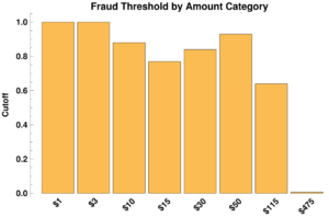
For small dollar amounts, the optimal cutoff was found to be essentially infinite. This makes some sense, as it means that, in transactions less than our cost of intervention ($5), there are no cases for which our automated fraud screening algorithm should fire. How do we prevent fraudsters from realizing our dilemma and exploiting it? The answer is fairly simple: flag cases many small, sequential transactions in a short period of time. This can be done easily by a computer and has inconsequential cost once the system is in place.
Above $10 transactions, we begin to see some variation in the cutoff. This is perhaps due to a complex relationship between 1) fraud depending on the transaction amount 2) the intrinsic ability of the machine learning to classify this particular data set, and 3) the cost-benefit for transactions within each bin.
Importantly, for large purchases (>$475), the threshold drops dramatically. It is fairly easy to understand: the possibility of having to absorb the cost of a high value transaction outweigh the cost of the intervention.
Most importantly, the net benefit with this approach is $365,000 – a net gain of $50,000 (compared to $315,000)!
In this post, I attempted to show the value of better classification methodologies, as well as the importance of taking into account economic considerations. This comprehensive approach that is more in tune with the realities of the business world.
The cost-benefit approach allows stakeholders to see the benefit of Advanced Analytics. Furthermore, this analysis forms a baseline for evaluating business improvement – such as understanding how the bottom line changes as a result of:
- changing parameters such as the cost of intervention (“What If” scenarios),
- the evaluation of the value of information by way of including/excluding certain predictors, and
- the inclusion of new terms, such as customer frustration.
and numerous other factors which may factor into making the best decision possible.
Works Cited
1. Kaggle https://www.kaggle.com/datasets/mlg-ulb/creditcardfraud